Power analysis based on a fitted scDesignPop marginal model

Chris Dong

Department of Statistics and Data Science, University of California, Los Angeles
cycd@g.ucla.edu

Yihui Cen

Department of Computational Medicine, University of California, Los Angeles
yihuicen@g.ucla.edu

23 January 2026

Introduction

scDesignPop provides power analysis tools at cell-type-specific level. Since fitted marginal models can be obtained by users already for generating synthetic datasets, the tutorial here is about how to conduct the power analysis on the basis of the marginal model files.

Library and data preparation

Here, we load the pre-saved marginal_list object to obtain the fitted marginal model of gene ENSG00000163221 (S100A12) for simplicity.

library(scDesignPop)
library(SingleCellExperiment)

data("marginal_list_sel")
summary(marginal_list_sel$ENSG00000163221$fit)
#>  Family: nbinom2  ( log )
#> Formula:          
#> response ~ (1 | indiv) + cell_type + `1:153337943` + `1:153337943`:cell_type
#> Data: res_list[["dmat_df"]]
#> 
#>       AIC       BIC    logLik -2*log(L)  df.resid 
#>   11088.7   11158.3   -5534.4   11068.7      7801 
#> 
#> Random effects:
#> 
#> Conditional model:
#>  Groups Name        Variance Std.Dev.
#>  indiv  (Intercept) 0.08141  0.2853  
#> Number of obs: 7811, groups:  indiv, 40
#> 
#> Dispersion parameter for nbinom2 family (): 1.15 
#> 
#> Conditional model:
#>                               Estimate Std. Error z value Pr(>|z|)    
#> (Intercept)                    1.80392    0.07763  23.237   <2e-16 ***
#> cell_typemononc               -4.65391    0.22215 -20.949   <2e-16 ***
#> cell_typebmem                 -5.96487    0.31401 -18.996   <2e-16 ***
#> cell_typecd4nc                -6.44683    0.22816 -28.256   <2e-16 ***
#> `1:153337943`                 -0.02273    0.08603  -0.264    0.792    
#> cell_typemononc:`1:153337943` -0.15160    0.27980  -0.542    0.588    
#> cell_typebmem:`1:153337943`   -0.55004    0.39328  -1.399    0.162    
#> cell_typecd4nc:`1:153337943`  -0.16812    0.29164  -0.576    0.564    
#> ---
#> Signif. codes:  0 '***' 0.001 '**' 0.01 '*' 0.05 '.' 0.1 ' ' 1

Performing power analysis

Given fitted marginal model, scDesignPop can perform simulation-based power analysis for a specific gene-SNP pair across selected cell types using the runPowerAnalysis function. Based on the previous naming of covariates, we specify the fitted snpid as "1:153337943", the name of the column for fixed cell state effect and random individual effect as "cell_type" and "indiv" in the input parameters. To check these namings, we can call the covariate data frame using marginal_list_sel[["ENSG00000163221"]]$fit$frame. The selected cell types for testing are specified in cellstate_vector and have to be consistent with the covariate data frame.

Particarly, parameters snp_number and gene_number are used to account for multiple testing correction with Bonferroni correction. Parameter methods is used to specify the marginal eQTL model from c("nb", "poisson", "gaussian", "pseudoBulkLinear"). Parameter nindivs and ncells are used to specify the number of individuals and number of cells per individual, from which we can analyze the performance of power analysis and find the optimal setting. Here, we set power_nsim = 1000 to increase the number of simulations so we can calculate power with a higher resolution. Using power_nsim = 100 in default or smaller values can reduce the computation time cost.

set.seed(123)
power_data <- runPowerAnalysis(marginal_list = marginal_list_sel,
                               marginal_model = "nb",
                               geneid = "ENSG00000163221",
                               snpid = "1:153337943",
                               celltype_colname = "cell_type",
                               celltype_vector = c("bmem", "monoc"),
                               indiv_colname = "indiv",
                               methods = c("poisson","pseudoBulkLinear"),
                               nindivs = c(50, 200),
                               ncells = c(10, 50),
                               alpha = 0.05,
                               power_nsim = 1000,
                               snp_number = 10,
                               gene_number = 800,
                               CI_nsim = 1000,
                               CI_conf = 0.05,
                               ncores = 25)
#> [1] -4.160949
#> [1] -0.5727631
#> [1] 1.803924
#> [1] -0.02272728
#> [1] -4.160949
#> [1] -0.5727631
#> [1] 1.803924
#> [1] -0.02272728

Visualization of power results

The power analysis results can be visualized using the visualizePowerCurve function. The cell type names in the cellstate_vector must be included in the above power analysis.

visualizePowerCurve(power_result = power_data,
                    celltype_vector = c("bmem", "monoc"),
                    x_axis = "nindiv",
                    y_facet = "ncell",
                    col_group = "method",
                    geneid = "ENSG00000163221",
                    snpid = "1:153337943")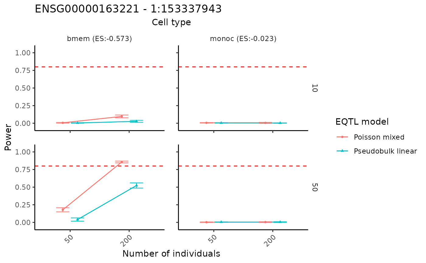

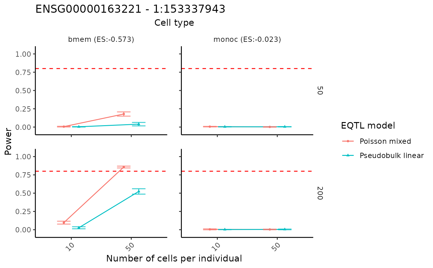
By swaping the x and y axis, we can show the result in a different way.

visualizePowerCurve(power_result = power_data,
                    celltype_vector = c("bmem", "monoc"),
                    x_axis = "ncell",
                    y_facet = "nindiv",
                    col_group = "method",
                    geneid = "ENSG00000163221",
                    snpid = "1:153337943")