Modeling batch effect in population-scale scRNA-seq data
Chris Dong
Department of Statistics and Data Science, University of California, Los Angelescycd@g.ucla.edu
Yihui Cen
Department of Computational Medicine, University of California, Los Angelesyihuicen@g.ucla.edu
13 February 2026
Source:vignettes/scDesignPop-batch-effect.Rmd
scDesignPop-batch-effect.Rmd
library(scDesignPop)
library(SingleCellExperiment)
library(SummarizedExperiment)
library(ggplot2)
theme_set(theme_bw())
Introduction
scDesignPop can model population-scale scRNA-seq data with batch covariates and enables simulation of datasets under user-specified batch effects, including scenarios in which batch effects are added or removed.
Library and data preparation
Here, we use an example SingleCellExperiment object
example_sce with 1000 genes and 7811 cells and an example
eQTL genotype dataframe example_eqtlgeno to demonstrate the
main tutorial. These two objects contains the gene expression and SNP
genotypes of 40 anonymized individuals while the eQTL genotype dataframe
provides 2826 putative cell-type-specific eQTLs.
library(scDesignPop)
library(SingleCellExperiment)
library(SummarizedExperiment)
library(ggplot2)

data("example_sce")
data("example_eqtlgeno")
The example_sce object also includes a pseudo-batch
covariate, where batch labels are randomly assigned to the 40
individuals at the individual level and applied to all cells belonging
to each individual.
colData(example_sce)
#> DataFrame with 7811 rows and 5 columns
#>            indiv cell_type       sex       age    batch
#>      <character>  <factor> <integer> <integer> <factor>
#> 1          SAMP1     cd4nc         2        65        1
#> 2          SAMP1     cd4nc         2        65        1
#> 3          SAMP1     cd4nc         2        65        1
#> 4          SAMP1     cd4nc         2        65        1
#> 5          SAMP1     cd4nc         2        65        1
#> ...          ...       ...       ...       ...      ...
#> 7807      SAMP14     monoc         1        87        1
#> 7808      SAMP14     bmem          1        87        1
#> 7809      SAMP14     bmem          1        87        1
#> 7810      SAMP14     bmem          1        87        1
#> 7811      SAMP14     bmem          1        87        1
Fitting batch effects
Step 1: construct a data list
To run scDesignPop, a list of data is required as input. This is done
using the constructDataPop function. A
SingleCellExperiment object and an eqtlgeno
dataframe are the two main inputs needed. The eqtlgeno
dataframe consists of eQTL annotations (it must have cell state, gene,
SNP, chromosome, and position columns at a minimum), and genotypes
across individuals (columns) for every SNP (rows). The structure of an
example eqtlgeno dataframe is given below.
data_list <- constructDataPop(
    sce = example_sce,
    eqtlgeno_df = example_eqtlgeno,
    new_covariate = as.data.frame(colData(example_sce)),
    overlap_features = NULL,
    sampid_vec = NULL,
    copula_variable = "cell_type",
    slot_name = "counts",
    snp_mode = "single",
    celltype_colname = "cell_type",
    feature_colname = "gene_id",
    snp_colname = "snp_id",
    loc_colname = "POS",
    chrom_colname = "CHR",
    indiv_colname = "indiv",
    prune_thres = 0.9
    )
Step 2: fit marginal model
Next, a marginal model is specified to fit each gene using the
fitMarginalPop function.
Here we use a Negative Binominal as the parametric model using
"nb". Since we want to include the batch effect modeling,
we specify mean_formula = "(1|indiv) + cell_type + batch.
Here, we use pseudo-batches to show how scDesignPop can model and alter
the batch effects.
marginal_list <- fitMarginalPop(
    data_list = data_list,
    mean_formula = "(1|indiv) + cell_type + batch",
    model_family = "nb",
    interact_colnames = "cell_type",
    parallelization = "pbmcapply",
    n_threads = 20L,
    loc_colname = "POS",
    snp_colname = "snp_id",
    celltype_colname = "cell_type",
    indiv_colname = "indiv",
    filter_snps = TRUE,
    snpvar_thres = 0,
    force_formula = FALSE,
    data_maxsize = 1
    )
Step 3: fit a Gaussian copula
The third step is to fit a Gaussian copula using the
fitCopulaPop function.
set.seed(123, kind = "L'Ecuyer-CMRG")

copula_fit <- fitCopulaPop(
    sce = example_sce,
    assay_use = "counts",
    input_data = data_list[["new_covariate"]],
    marginal_list = marginal_list,
    family_use = "nb",
    copula = "gaussian",
    n_cores = 2L,
    parallelization = "mcmapply"
    )

RNGkind("Mersenne-Twister")  # reset
Step 4: extract parameters
The fourth step is to compute the mean, sigma, and zero probability
parameters using the extractParaPop function.
para_new <- extractParaPop(
    sce = example_sce,
    assay_use = "counts",
    marginal_list = marginal_list,
    n_cores = 2L,
    family_use = "nb",
    indiv_colname = "indiv",
    new_covariate = data_list[["new_covariate"]],
    new_eqtl_geno_list = data_list[["eqtl_geno_list"]],
    data = data_list[["covariate"]],
    parallelization = "pbmcmapply"
    )
Step 5: simulate counts
The fifth step is to simulate counts using the
simuNewPop function.
set.seed(123)

newcount_mat <- simuNewPop(
    sce = example_sce,
    mean_mat = para_new[["mean_mat"]],
    sigma_mat = para_new[["sigma_mat"]],
    zero_mat = para_new[["zero_mat"]],
    quantile_mat = NULL,
    copula_list = copula_fit[["copula_list"]],
    n_cores = 2L,
    family_use = "nb",
    nonnegative = TRUE,
    input_data = data_list[["covariate"]],
    new_covariate = data_list[["new_covariate"]],
    important_feature = copula_fit[["important_feature"]],
    filtered_gene = data_list[["filtered_gene"]],
    parallelization = "pbmcmapply"
)Set new batch effects
Step 1: set new batch effect sizes in marginal models
Check the rank of the batch effect sizes in the marginal
distributions. Here, we take the gene ENSG00000023902 as
example since every gene are fitted using the same formula.
marginal_list$ENSG00000023902$fit
#> Formula:          response ~ (1 | indiv) + cell_type + batch + `1:150133323` +
#>     `1:150133323`:cell_type
#> Data: res_list[["dmat_df"]]
#>       AIC       BIC    logLik  df.resid
#>  8048.619  8125.215 -4013.309      7800
#> Random-effects (co)variances:
#>
#> Conditional model:
#>  Groups Name        Std.Dev.
#>  indiv  (Intercept) 0.1984
#>
#> Number of obs: 7811 / Conditional model: indiv, 40
#>
#> Dispersion parameter for nbinom2 family (): 1.64
#>
#> Fixed Effects:
#>
#> Conditional model:
#>                   (Intercept)                cell_typemononc
#>                      -0.95994                        0.33161
#>                 cell_typebmem                 cell_typecd4nc
#>                      -0.68688                       -1.64664
#>                        batch2                  `1:150133323`
#>                      -0.18556                        0.21056
#> cell_typemononc:`1:150133323`    cell_typebmem:`1:150133323`
#>                      -0.15846                       -0.05042
#>  cell_typecd4nc:`1:150133323`
#>                      -0.12240
After the ranks of the batch effects are obtained, set a new value to the gene marginal models and check the summary report again.
marginal_list_diff <- lapply(marginal_list, function(x) {
  val <- rnorm(1, mean = 10, sd = 2) # set zero for batch effect removal
  x$fit$fit$par[5] <- val
  x$fit$fit$parfull[5] <- val
  x$fit$sdr$par.fixed[5] <- val
  x
})

marginal_list_diff$ENSG00000023902$fit
#> Formula:          response ~ (1 | indiv) + cell_type + batch + `1:150133323` +
#>     `1:150133323`:cell_type
#> Data: res_list[["dmat_df"]]
#>       AIC       BIC    logLik  df.resid
#>  8048.619  8125.215 -4013.309      7800
#> Random-effects (co)variances:
#>
#> Conditional model:
#>  Groups Name        Std.Dev.
#>  indiv  (Intercept) 0.1984
#>
#> Number of obs: 7811 / Conditional model: indiv, 40
#>
#> Dispersion parameter for nbinom2 family (): 1.64
#>
#> Fixed Effects:
#>
#> Conditional model:
#>                   (Intercept)                cell_typemononc
#>                      -0.95994                        0.33161
#>                 cell_typebmem                 cell_typecd4nc
#>                      -0.68688                       -1.64664
#>                        batch2                  `1:150133323`
#>                       6.00619                        0.21056
#> cell_typemononc:`1:150133323`    cell_typebmem:`1:150133323`
#>                      -0.15846                       -0.05042
#>  cell_typecd4nc:`1:150133323`
#>                      -0.12240
Step 2: re-extract the parameters
para_new_diff <- extractParaPop(
    sce = example_sce,
    assay_use = "counts",
    marginal_list = marginal_list_diff,
    n_cores = 2L,
    family_use = "nb",
    indiv_colname = "indiv",
    new_covariate = data_list[["new_covariate"]],
    new_eqtl_geno_list = data_list[["eqtl_geno_list"]],
    data = data_list[["covariate"]],
    parallelization = "pbmcmapply"
    )
Step 3: simulate counts with batch effects
set.seed(123)

newcount_mat_diff <- simuNewPop(
    sce = example_sce,
    mean_mat = para_new_diff[["mean_mat"]],
    sigma_mat = para_new_diff[["sigma_mat"]],
    zero_mat = para_new_diff[["zero_mat"]],
    quantile_mat = NULL,
    copula_list = copula_fit[["copula_list"]],
    n_cores = 2L,
    family_use = "nb",
    nonnegative = TRUE,
    input_data = data_list[["covariate"]],
    new_covariate = data_list[["new_covariate"]],
    important_feature = copula_fit[["important_feature"]],
    filtered_gene = data_list[["filtered_gene"]],
    parallelization = "pbmcmapply"
)Visualization
The simulated data can be visualized using a UMAP plot as follows.
logcounts(simu_sce) <- log1p(counts(simu_sce))
logcounts(simu_sce_diff) <- log1p(counts(simu_sce_diff))
set.seed(123)
compare_figure <- scDesignPop::plotReducedDimPop(
    ref_sce = example_sce,
    sce_list = list(simu_sce, simu_sce_diff),
    name_vec = c("Reference", "w/o batch effects", "w/ batch effects"),
    assay_use = "logcounts",
    if_plot = TRUE,
    color_by = "batch", point_size = 0.1,
    n_pc = 30)
plot(compare_figure$p_umap)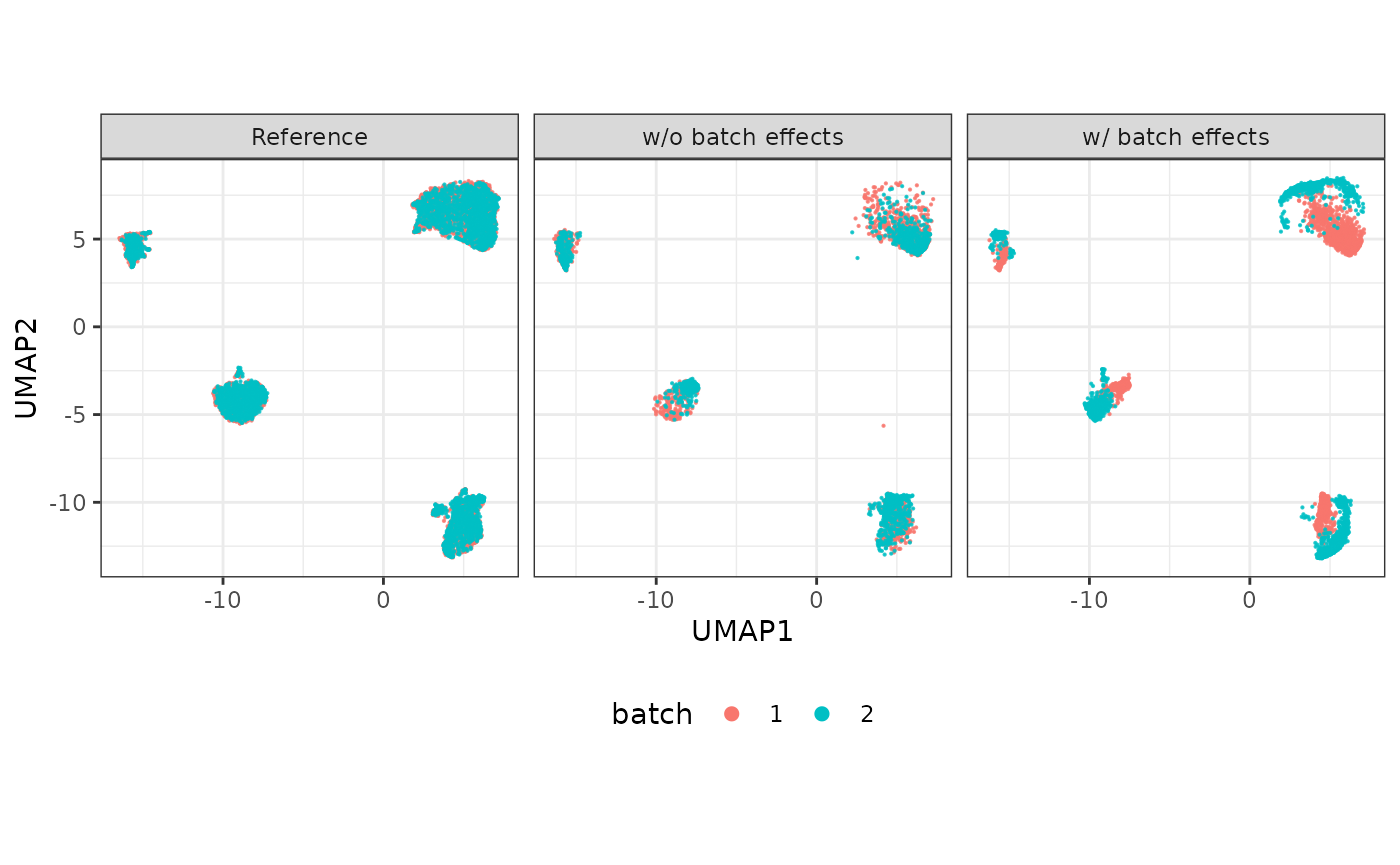
Session information
sessionInfo()
#> R version 4.2.3 (2023-03-15)
#> Platform: x86_64-pc-linux-gnu (64-bit)
#> Running under: Ubuntu 22.04.5 LTS
#>
#> Matrix products: default
#> BLAS:   /usr/lib/x86_64-linux-gnu/openblas-pthread/libblas.so.3
#> LAPACK: /usr/lib/x86_64-linux-gnu/openblas-pthread/libopenblasp-r0.3.20.so
#>
#> locale:
#>  [1] LC_CTYPE=en_US.UTF-8       LC_NUMERIC=C
#>  [3] LC_TIME=en_US.UTF-8        LC_COLLATE=en_US.UTF-8
#>  [5] LC_MONETARY=en_US.UTF-8    LC_MESSAGES=en_US.UTF-8
#>  [7] LC_PAPER=en_US.UTF-8       LC_NAME=C
#>  [9] LC_ADDRESS=C               LC_TELEPHONE=C
#> [11] LC_MEASUREMENT=en_US.UTF-8 LC_IDENTIFICATION=C
#>
#> attached base packages:
#> [1] stats4    stats     graphics  grDevices utils     datasets  methods
#> [8] base
#>
#> other attached packages:
#>  [1] ggplot2_3.5.2               SingleCellExperiment_1.20.1
#>  [3] SummarizedExperiment_1.28.0 Biobase_2.58.0
#>  [5] GenomicRanges_1.50.2        GenomeInfoDb_1.34.9
#>  [7] IRanges_2.32.0              S4Vectors_0.36.2
#>  [9] BiocGenerics_0.44.0         MatrixGenerics_1.10.0
#> [11] matrixStats_1.1.0           scDesignPop_0.0.0.9010
#> [13] BiocStyle_2.26.0
#>
#> loaded via a namespace (and not attached):
#>  [1] viridis_0.6.5          sass_0.4.10            jsonlite_2.0.0
#>  [4] viridisLite_0.4.2      splines_4.2.3          RhpcBLASctl_0.23-42
#>  [7] bslib_0.9.0            assertthat_0.2.1       BiocManager_1.30.25
#> [10] GenomeInfoDbData_1.2.9 yaml_2.3.10            numDeriv_2016.8-1.1
#> [13] pillar_1.10.2          lattice_0.22-6         glue_1.8.0
#> [16] digest_0.6.37          RColorBrewer_1.1-3     XVector_0.38.0
#> [19] glmmTMB_1.1.9          minqa_1.2.8            htmltools_0.5.8.1
#> [22] Matrix_1.6-5           pkgconfig_2.0.3        bookdown_0.43
#> [25] zlibbioc_1.44.0        mvtnorm_1.3-3          scales_1.4.0
#> [28] lme4_1.1-35.3          tibble_3.2.1           mgcv_1.9-1
#> [31] generics_0.1.4         farver_2.1.2           withr_3.0.2
#> [34] cachem_1.1.0           pbapply_1.7-2          TMB_1.9.11
#> [37] cli_3.6.5              magrittr_2.0.3         evaluate_1.0.3
#> [40] fs_1.6.6               nlme_3.1-164           MASS_7.3-58.2
#> [43] textshaping_0.4.0      tools_4.2.3            lifecycle_1.0.4
#> [46] DelayedArray_0.24.0    irlba_2.3.5.1          compiler_4.2.3
#> [49] pkgdown_2.2.0          jquerylib_0.1.4        pbmcapply_1.5.1
#> [52] systemfonts_1.2.3      rlang_1.1.6            grid_4.2.3
#> [55] RCurl_1.98-1.17        nloptr_2.2.1           rstudioapi_0.17.1
#> [58] RcppAnnoy_0.0.22       htmlwidgets_1.6.4      labeling_0.4.3
#> [61] bitops_1.0-9           rmarkdown_2.27         boot_1.3-30
#> [64] codetools_0.2-20       gtable_0.3.6           R6_2.6.1
#> [67] gridExtra_2.3          knitr_1.50             dplyr_1.1.4
#> [70] fastmap_1.2.0          uwot_0.2.3             ragg_1.5.0
#> [73] desc_1.4.3             parallel_4.2.3         Rcpp_1.0.14
#> [76] vctrs_0.6.5            tidyselect_1.2.1       xfun_0.52