scDesignPop Quickstart
Chris Dong
Department of Statistics and Data Science, University of California, Los Angelescycd@g.ucla.edu
Yihui Cen
Department of Computational Medicine, University of California, Los Angelesyihuicen@g.ucla.edu
13 February 2026
Source:vignettes/scDesignPop.Rmd
scDesignPop.Rmd
library(scDesignPop)
library(SingleCellExperiment)
library(SummarizedExperiment)
library(ggplot2)
theme_set(theme_bw())
Introduction
scDesignPop is a simulator for population-scale single-cell RNA-sequencing (scRNA-seq) data. For more information, please check the Articles on our website: (https://chrisycd.github.io/scDesignPop/docs/index.html).
Library and data preparation
Here, we use an example SingleCellExperiment object
example_sce with 1000 genes and 7811 cells and an example
eQTL genotype dataframe example_eqtlgeno to demonstrate the
main tutorial. These two objects contains the gene expression and SNP
genotypes of 40 anonymized individuals while the eQTL genotype dataframe
provides 2826 putative cell-type-specific eQTLs.
library(scDesignPop)
library(SingleCellExperiment)
library(SummarizedExperiment)
library(ggplot2)

data("example_sce")
data("example_eqtlgeno")

example_sce
#> class: SingleCellExperiment
#> dim: 1000 7811
#> metadata(0):
#> assays(2): counts logcounts
#> rownames(1000): ENSG00000023902 ENSG00000027869 ... ENSG00000254709
#>   ENSG00000272216
#> rowData names(0):
#> colnames: NULL
#> colData names(5): indiv cell_type sex age batch
#> reducedDimNames(0):
#> mainExpName: RNA
#> altExpNames(0):
head(example_eqtlgeno[,1:8])
#> # A tibble: 6 × 8
#>   cell_type gene_id         snp_id        CHR       POS SAMP1 SAMP2 SAMP3
#>   <chr>     <chr>           <chr>       <dbl>     <dbl> <dbl> <dbl> <dbl>
#> 1 cd4nc     ENSG00000023902 1:150133323     1 150133323     0     0     0
#> 2 cd8nc     ENSG00000023902 1:150159616     1 150159616     2     2     1
#> 3 cd4nc     ENSG00000027869 1:156693018     1 156693018     0     0     0
#> 4 cd4nc     ENSG00000028137 1:12192270      1  12192270     2     2     1
#> 5 cd8nc     ENSG00000028137 1:12267999      1  12267999     2     1     1
#> 6 nk        ENSG00000028137 1:12267999      1  12267999     1     0     1
dim(example_eqtlgeno)
#> [1] 2826   45
Modeling and simulation
Step 1: construct a data list
To run scDesignPop, a list of data is required as input. This is done
using the constructDataPop function. A
SingleCellExperiment object and an eqtlgeno
dataframe are the two main inputs needed. The eqtlgeno
dataframe consists of eQTL annotations (it must have cell state, gene,
SNP, chromosome, and position columns at a minimum), and genotypes
across individuals (columns) for every SNP (rows). The structure of an
example eqtlgeno dataframe is also given below.
head(example_eqtlgeno)
#> # A tibble: 6 × 45
#>   cell_type gene_id      snp_id   CHR    POS SAMP1 SAMP2 SAMP3 SAMP4 SAMP5 SAMP6
#>   <chr>     <chr>        <chr>  <dbl>  <dbl> <dbl> <dbl> <dbl> <dbl> <dbl> <dbl>
#> 1 cd4nc     ENSG0000002… 1:150…     1 1.50e8     0     0     0     0     0     1
#> 2 cd8nc     ENSG0000002… 1:150…     1 1.50e8     2     2     1     1     1     2
#> 3 cd4nc     ENSG0000002… 1:156…     1 1.57e8     0     0     0     0     1     0
#> 4 cd4nc     ENSG0000002… 1:121…     1 1.22e7     2     2     1     1     1     0
#> 5 cd8nc     ENSG0000002… 1:122…     1 1.23e7     2     1     1     2     1     2
#> 6 nk        ENSG0000002… 1:122…     1 1.23e7     1     0     1     0     0     1
#> # ℹ 34 more variables: SAMP7 <dbl>, SAMP8 <dbl>, SAMP9 <dbl>, SAMP10 <dbl>,
#> #   SAMP11 <dbl>, SAMP12 <dbl>, SAMP13 <dbl>, SAMP14 <dbl>, SAMP15 <dbl>,
#> #   SAMP16 <dbl>, SAMP17 <dbl>, SAMP18 <dbl>, SAMP19 <dbl>, SAMP20 <dbl>,
#> #   SAMP21 <dbl>, SAMP22 <dbl>, SAMP23 <dbl>, SAMP24 <dbl>, SAMP25 <dbl>,
#> #   SAMP26 <dbl>, SAMP27 <dbl>, SAMP28 <dbl>, SAMP29 <dbl>, SAMP30 <dbl>,
#> #   SAMP31 <dbl>, SAMP32 <dbl>, SAMP33 <dbl>, SAMP34 <dbl>, SAMP35 <dbl>,
#> #   SAMP36 <dbl>, SAMP37 <dbl>, SAMP38 <dbl>, SAMP39 <dbl>, SAMP40 <dbl>
data_list <- constructDataPop(
    sce = example_sce,
    eqtlgeno_df = example_eqtlgeno,
    new_covariate = as.data.frame(colData(example_sce)),
    overlap_features = NULL,
    sampid_vec = NULL,
    copula_variable = "cell_type",
    slot_name = "counts",
    snp_mode = "single",
    celltype_colname = "cell_type",
    feature_colname = "gene_id",
    snp_colname = "snp_id",
    loc_colname = "POS",
    chrom_colname = "CHR",
    indiv_colname = "indiv",
    prune_thres = 0.9
    )
Step 2: fit marginal model
Next, a marginal model is specified to fit each gene using the
fitMarginalPop function.
Here we use a Negative Binominal as the parametric model using
"nb".
marginal_list <- fitMarginalPop(
    data_list = data_list,
    mean_formula = "(1|indiv) + cell_type",
    model_family = "nb",
    interact_colnames = "cell_type",
    parallelization = "pbmcapply",
    n_threads = 20L,
    loc_colname = "POS",
    snp_colname = "snp_id",
    celltype_colname = "cell_type",
    indiv_colname = "indiv",
    filter_snps = TRUE,
    snpvar_thres = 0,
    force_formula = FALSE,
    data_maxsize = 1
    )
Step 3: fit a Gaussian copula
The third step is to fit a Gaussian copula using the
fitCopulaPop function.
set.seed(123, kind = "L'Ecuyer-CMRG")

copula_fit <- fitCopulaPop(
    sce = example_sce,
    assay_use = "counts",
    input_data = data_list[["new_covariate"]],
    marginal_list = marginal_list,
    family_use = "nb",
    copula = "gaussian",
    n_cores = 2L,
    parallelization = "mcmapply"
    )

RNGkind("Mersenne-Twister")  # reset
Step 4: extract parameters
The fourth step is to compute the mean, sigma, and zero probability
parameters using the extractParaPop function.
para_new <- extractParaPop(
    sce = example_sce,
    assay_use = "counts",
    marginal_list = marginal_list,
    n_cores = 2L,
    family_use = "nb",
    indiv_colname = "indiv",
    new_covariate = data_list[["new_covariate"]],
    new_eqtl_geno_list = data_list[["eqtl_geno_list"]],
    data = data_list[["covariate"]],
    parallelization = "pbmcmapply"
    )
Step 5: simulate counts
The fifth step is to simulate counts using the
simuNewPop function.
set.seed(123)

newcount_mat <- simuNewPop(
    sce = example_sce,
    mean_mat = para_new[["mean_mat"]],
    sigma_mat = para_new[["sigma_mat"]],
    zero_mat = para_new[["zero_mat"]],
    quantile_mat = NULL,
    copula_list = copula_fit[["copula_list"]],
    n_cores = 2L,
    family_use = "nb",
    nonnegative = TRUE,
    input_data = data_list[["covariate"]],
    new_covariate = data_list[["new_covariate"]],
    important_feature = copula_fit[["important_feature"]],
    filtered_gene = data_list[["filtered_gene"]],
    parallelization = "pbmcmapply"
)Visualization
The simulated data can be visualized using a UMAP plot as follows.
logcounts(simu_sce) <- log1p(counts(simu_sce))
set.seed(123)
compare_figure <- scDesignPop::plotReducedDimPop(
    ref_sce = example_sce,
    sce_list = list(simu_sce),
    name_vec = c("Reference", "scDesignPop"),
    assay_use = "logcounts",
    if_plot = TRUE,
    color_by = "cell_type", point_size = 1,
    n_pc = 30)
plot(compare_figure$p_umap)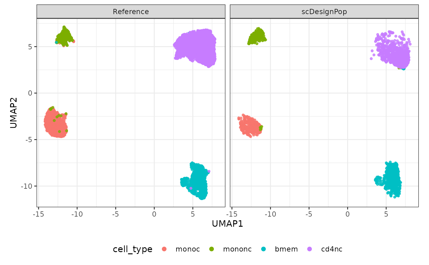
Session information
sessionInfo()
#> R version 4.2.3 (2023-03-15)
#> Platform: x86_64-pc-linux-gnu (64-bit)
#> Running under: Ubuntu 22.04.5 LTS
#>
#> Matrix products: default
#> BLAS:   /usr/lib/x86_64-linux-gnu/openblas-pthread/libblas.so.3
#> LAPACK: /usr/lib/x86_64-linux-gnu/openblas-pthread/libopenblasp-r0.3.20.so
#>
#> locale:
#>  [1] LC_CTYPE=en_US.UTF-8       LC_NUMERIC=C
#>  [3] LC_TIME=en_US.UTF-8        LC_COLLATE=en_US.UTF-8
#>  [5] LC_MONETARY=en_US.UTF-8    LC_MESSAGES=en_US.UTF-8
#>  [7] LC_PAPER=en_US.UTF-8       LC_NAME=C
#>  [9] LC_ADDRESS=C               LC_TELEPHONE=C
#> [11] LC_MEASUREMENT=en_US.UTF-8 LC_IDENTIFICATION=C
#>
#> attached base packages:
#> [1] stats4    stats     graphics  grDevices utils     datasets  methods
#> [8] base
#>
#> other attached packages:
#>  [1] ggplot2_3.5.2               SingleCellExperiment_1.20.1
#>  [3] SummarizedExperiment_1.28.0 Biobase_2.58.0
#>  [5] GenomicRanges_1.50.2        GenomeInfoDb_1.34.9
#>  [7] IRanges_2.32.0              S4Vectors_0.36.2
#>  [9] BiocGenerics_0.44.0         MatrixGenerics_1.10.0
#> [11] matrixStats_1.1.0           scDesignPop_0.0.0.9010
#> [13] BiocStyle_2.26.0
#>
#> loaded via a namespace (and not attached):
#>  [1] viridis_0.6.5          sass_0.4.10            jsonlite_2.0.0
#>  [4] viridisLite_0.4.2      splines_4.2.3          RhpcBLASctl_0.23-42
#>  [7] bslib_0.9.0            assertthat_0.2.1       BiocManager_1.30.25
#> [10] GenomeInfoDbData_1.2.9 yaml_2.3.10            numDeriv_2016.8-1.1
#> [13] pillar_1.10.2          lattice_0.22-6         glue_1.8.0
#> [16] digest_0.6.37          RColorBrewer_1.1-3     XVector_0.38.0
#> [19] glmmTMB_1.1.9          minqa_1.2.8            htmltools_0.5.8.1
#> [22] Matrix_1.6-5           pkgconfig_2.0.3        bookdown_0.43
#> [25] zlibbioc_1.44.0        mvtnorm_1.3-3          scales_1.4.0
#> [28] lme4_1.1-35.3          tibble_3.2.1           mgcv_1.9-1
#> [31] generics_0.1.4         farver_2.1.2           withr_3.0.2
#> [34] cachem_1.1.0           pbapply_1.7-2          TMB_1.9.11
#> [37] cli_3.6.5              magrittr_2.0.3         evaluate_1.0.3
#> [40] fs_1.6.6               nlme_3.1-164           MASS_7.3-58.2
#> [43] textshaping_0.4.0      tools_4.2.3            lifecycle_1.0.4
#> [46] DelayedArray_0.24.0    irlba_2.3.5.1          compiler_4.2.3
#> [49] pkgdown_2.2.0          jquerylib_0.1.4        pbmcapply_1.5.1
#> [52] systemfonts_1.2.3      rlang_1.1.6            grid_4.2.3
#> [55] RCurl_1.98-1.17        nloptr_2.2.1           rstudioapi_0.17.1
#> [58] RcppAnnoy_0.0.22       htmlwidgets_1.6.4      labeling_0.4.3
#> [61] bitops_1.0-9           rmarkdown_2.27         boot_1.3-30
#> [64] codetools_0.2-20       gtable_0.3.6           R6_2.6.1
#> [67] gridExtra_2.3          knitr_1.50             dplyr_1.1.4
#> [70] utf8_1.2.5             fastmap_1.2.0          uwot_0.2.3
#> [73] ragg_1.5.0             desc_1.4.3             parallel_4.2.3
#> [76] Rcpp_1.0.14            vctrs_0.6.5            tidyselect_1.2.1
#> [79] xfun_0.52