Model linear dynamic eQTL effects in continuous cell states
Chris Dong
Department of Statistics and Data Science, University of California, Los Angelescycd@g.ucla.edu
Yihui Cen
Department of Computational Medicine, University of California, Los Angelesyihuicen@g.ucla.edu
13 February 2026
Source:vignettes/scDesignPop-dynamic-eQTL.Rmd
scDesignPop-dynamic-eQTL.Rmd
library(scDesignPop)
library(SingleCellExperiment)
library(SummarizedExperiment)
library(scater)
theme_set(theme_bw())
Introduction
scDesignPop can also be extended to other eQTL effects. Here we show how scDesignPop can also model linear dynamic eQTL effects in continuous cell states to mimick the real data better.
Library and data preparation
Here, we use a subset of the B cells from OneK1K cohort as example.
We load an example SingleCellExperiment object example_sce
with 817 genes and 3726 cells and an example eQTL genotype dataframe
example_eqtlgeno to demonstrate the main tutorial. These
two objects contains the gene expression and SNP genotypes of 100
anonymized individuals while the eQTL genotype dataframe provides 2406
putative cell-type-specific eQTLs.
library(scDesignPop)
library(SingleCellExperiment)
library(SummarizedExperiment)
library(scater)

data("example_sce_Bcell")
data("example_eqtlgeno_Bcell")
head(colData(example_sce_Bcell))
#> DataFrame with 6 rows and 5 columns
#>                    cell_type    indiv      sex       age slingPseudotime_1
#>                     <factor> <factor> <factor> <integer>         <numeric>
#> AAAGATGGTTATGCGT-1      bin    SAMP68        1        69          0.215705
#> AACTCAGGTCCGCTGA-1      bin    SAMP68        1        69          0.835651
#> AAGTCTGTCGTACGGC-1      bin    SAMP68        1        69          0.532256
#> ACACCGGCACCCTATC-1      bin    SAMP68        1        69          0.423183
#> ACGCCGAGTCAGAGGT-1      bmem   SAMP68        1        69          0.268401
#> ACTGAGTCAGGATCGA-1      bin    SAMP68        1        69          0.480905
Modeling and simulation
Step 1: construct a data list
scDesignPop can also be extended to other eQTL effects. Here we show
how scDesignPop can model dynamic eQTL effects in continuous cell states
as potential in-silico ground-truth. We only consider linear dynamic
eQTL effects here for simplicity. To run scDesignPop, a list of data is
required as input. This is done using the constructDataPop
function. A SingleCellExperiment object and an
eqtlgeno dataframe are the two main inputs needed. The
eqtlgeno dataframe consists of eQTL annotations (it must
have cell state, gene, SNP, chromosome, and position columns at a
minimum), and genotypes across individuals (columns) for every SNP
(rows). The structure of an example eqtlgeno dataframe is
given below.
data_list <- constructDataPop(
    sce = example_sce_Bcell,
    eqtlgeno_df = example_eqtlgeno_Bcell,
    new_covariate = as.data.frame(colData(example_sce_Bcell)),
    overlap_features = NULL,
    sampid_vec = NULL,
    copula_variable = "slingPseudotime_1",
    n_quantiles = 10,
    slot_name = "counts",
    snp_mode = "single",
    time_colname = "slingPseudotime_1",
    celltype_colname = "cell_type",
    feature_colname = "gene_id",
    snp_colname = "snp_id",
    loc_colname = "POS",
    chrom_colname = "CHR",
    indiv_colname = "indiv",
    prune_thres = 0.9
    )
Step 2: fit marginal model
Next, a marginal model is specified to fit each gene using the
fitMarginalPop function.
Here we use a Negative Binominal as the parametric model using
"nb".
marginal_list <- fitMarginalPop(
    data_list = data_list,
    mean_formula = "(1|indiv) + slingPseudotime_1",
    model_family = "nb",
    interact_colnames = c("slingPseudotime_1"),
    parallelization = "pbmcapply",
    n_threads = 20L,
    loc_colname = "POS",
    snp_colname = "snp_id",
    celltype_colname = "cell_type",
    indiv_colname = "indiv",
    filter_snps = TRUE,
    snpvar_thres = 0,
    force_formula = FALSE,
    data_maxsize = 1
    )
Step 3: fit a Gaussian copula
The third step is to fit a Gaussian copula using the
fitCopulaPop function.
set.seed(123, kind = "L'Ecuyer-CMRG")

copula_fit <- fitCopulaPop(
    sce = example_sce_Bcell,
    assay_use = "counts",
    input_data = data_list[["new_covariate"]],
    marginal_list = marginal_list,
    family_use = "nb",
    copula = "gaussian",
    n_cores = 2L,
    parallelization = "mcmapply"
    )

RNGkind("Mersenne-Twister")  # reset
Step 4: extract parameters
The fourth step is to compute the mean, sigma, and zero probability
parameters using the extractParaPop function.
para_new <- extractParaPop(
    sce = example_sce_Bcell,
    assay_use = "counts",
    marginal_list = marginal_list,
    n_cores = 2L,
    family_use = "nb",
    indiv_colname = "indiv",
    new_covariate = data_list[["new_covariate"]],
    new_eqtl_geno_list = data_list[["eqtl_geno_list"]],
    data = data_list[["covariate"]],
    parallelization = "pbmcmapply"
    )
Step 5: simulate counts
The fifth step is to simulate counts using the
simuNewPop function.
set.seed(123)

newcount_mat <- simuNewPop(
    sce = example_sce_Bcell,
    mean_mat = para_new[["mean_mat"]],
    sigma_mat = para_new[["sigma_mat"]],
    zero_mat = para_new[["zero_mat"]],
    quantile_mat = NULL,
    copula_list = copula_fit[["copula_list"]],
    n_cores = 2L,
    family_use = "nb",
    nonnegative = TRUE,
    input_data = data_list[["covariate"]],
    new_covariate = data_list[["new_covariate"]],
    important_feature = copula_fit[["important_feature"]],
    filtered_gene = data_list[["filtered_gene"]],
    parallelization = "pbmcmapply"
)Visualization using PHATE
The simulated data can be visualized using a UMAP plot as follows.
library(ggplot2)
library(phateR)

# run PHATE for reference data
ph <- phate(t(counts(example_sce_Bcell)))
#> Calculating PHATE...
#>   Running PHATE on 3726 observations and 817 variables.
#>   Calculating graph and diffusion operator...
#>     Calculating PCA...
#>     Calculated PCA in 0.27 seconds.
#>     Calculating KNN search...
#>     Calculated KNN search in 0.96 seconds.
#>     Calculating affinities...
#>     Calculated affinities in 0.02 seconds.
#>   Calculated graph and diffusion operator in 1.25 seconds.
#>   Calculating landmark operator...
#>     Calculating SVD...
#>     Calculated SVD in 0.23 seconds.
#>     Calculating KMeans...
#>     Calculated KMeans in 4.90 seconds.
#>   Calculated landmark operator in 5.56 seconds.
#>   Calculating optimal t...
#>     Automatically selected t = 18
#>   Calculated optimal t in 0.76 seconds.
#>   Calculating diffusion potential...
#>   Calculated diffusion potential in 0.15 seconds.
#>   Calculating metric MDS...
#>   Calculated metric MDS in 3.77 seconds.
#> Calculated PHATE in 11.49 seconds.
reducedDims(example_sce_Bcell) <- SimpleList(PHATE = ph$embedding)

# run PHATE for simulated data
ph_simu <- phate(t(counts(simu_sce_Bcell)))
#> Calculating PHATE...
#>   Running PHATE on 3726 observations and 817 variables.
#>   Calculating graph and diffusion operator...
#>     Calculating PCA...
#>     Calculated PCA in 0.26 seconds.
#>     Calculating KNN search...
#>     Calculated KNN search in 0.87 seconds.
#>     Calculating affinities...
#>     Calculated affinities in 0.02 seconds.
#>   Calculated graph and diffusion operator in 1.16 seconds.
#>   Calculating landmark operator...
#>     Calculating SVD...
#>     Calculated SVD in 0.24 seconds.
#>     Calculating KMeans...
#>     Calculated KMeans in 3.39 seconds.
#>   Calculated landmark operator in 4.03 seconds.
#>   Calculating optimal t...
#>     Automatically selected t = 15
#>   Calculated optimal t in 0.74 seconds.
#>   Calculating diffusion potential...
#>   Calculated diffusion potential in 0.13 seconds.
#>   Calculating metric MDS...
#>   Calculated metric MDS in 3.69 seconds.
#> Calculated PHATE in 9.77 seconds.
reducedDims(simu_sce_Bcell) <- SimpleList(PHATE = ph_simu$embedding)

# visualize
p <- ggplot(reducedDim(example_sce_Bcell),
            aes(PHATE1, PHATE2, color = example_sce_Bcell$slingPseudotime_1)) +
  ggrastr::rasterise(
    geom_point(size = 0.5),
    dpi = 300
  ) +
  labs(color = "Pseudotime") +
  theme_classic() +
  theme(plot.title = element_text(hjust = 0.5)) +
    ggtitle("Reference")

p_simu <- ggplot(reducedDim(simu_sce_Bcell),
                 aes(PHATE1, PHATE2,
                     color = colData(simu_sce_Bcell)$slingPseudotime_1)) +
  ggrastr::rasterise(
    geom_point(size = 0.5),
    dpi = 300
  ) +
  labs(color = "Pseudotime") +
  theme_classic() +
  theme(plot.title = element_text(hjust = 0.5)) +
    ggtitle("scDesignPop (Linear Dynamic eQTL)")

patchwork::wrap_plots(p, p_simu, ncol = 2)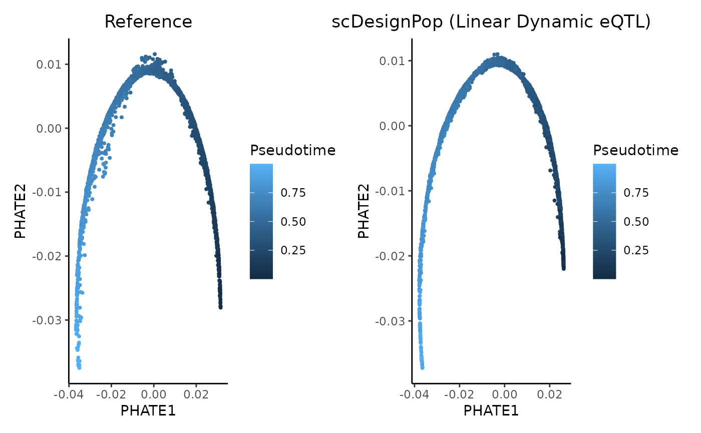
Session information
sessionInfo()
#> R version 4.2.3 (2023-03-15)
#> Platform: x86_64-pc-linux-gnu (64-bit)
#> Running under: Ubuntu 22.04.5 LTS
#>
#> Matrix products: default
#> BLAS:   /usr/lib/x86_64-linux-gnu/openblas-pthread/libblas.so.3
#> LAPACK: /usr/lib/x86_64-linux-gnu/openblas-pthread/libopenblasp-r0.3.20.so
#>
#> locale:
#>  [1] LC_CTYPE=en_US.UTF-8       LC_NUMERIC=C
#>  [3] LC_TIME=en_US.UTF-8        LC_COLLATE=en_US.UTF-8
#>  [5] LC_MONETARY=en_US.UTF-8    LC_MESSAGES=en_US.UTF-8
#>  [7] LC_PAPER=en_US.UTF-8       LC_NAME=C
#>  [9] LC_ADDRESS=C               LC_TELEPHONE=C
#> [11] LC_MEASUREMENT=en_US.UTF-8 LC_IDENTIFICATION=C
#>
#> attached base packages:
#> [1] stats4    stats     graphics  grDevices utils     datasets  methods
#> [8] base
#>
#> other attached packages:
#>  [1] phateR_1.0.7                Matrix_1.6-5
#>  [3] scater_1.26.1               ggplot2_3.5.2
#>  [5] scuttle_1.8.4               SingleCellExperiment_1.20.1
#>  [7] SummarizedExperiment_1.28.0 Biobase_2.58.0
#>  [9] GenomicRanges_1.50.2        GenomeInfoDb_1.34.9
#> [11] IRanges_2.32.0              S4Vectors_0.36.2
#> [13] BiocGenerics_0.44.0         MatrixGenerics_1.10.0
#> [15] matrixStats_1.1.0           scDesignPop_0.0.0.9010
#> [17] BiocStyle_2.26.0
#>
#> loaded via a namespace (and not attached):
#>  [1] nlme_3.1-164              bitops_1.0-9
#>  [3] fs_1.6.6                  RColorBrewer_1.1-3
#>  [5] rprojroot_2.1.1           numDeriv_2016.8-1.1
#>  [7] tools_4.2.3               TMB_1.9.11
#>  [9] bslib_0.9.0               R6_2.6.1
#> [11] irlba_2.3.5.1             vipor_0.4.7
#> [13] uwot_0.2.3                mgcv_1.9-1
#> [15] withr_3.0.2               ggrastr_1.0.2
#> [17] tidyselect_1.2.1          gridExtra_2.3
#> [19] compiler_4.2.3            textshaping_0.4.0
#> [21] cli_3.6.5                 BiocNeighbors_1.16.0
#> [23] Cairo_1.6-2               desc_1.4.3
#> [25] DelayedArray_0.24.0       labeling_0.4.3
#> [27] bookdown_0.43             sass_0.4.10
#> [29] scales_1.4.0              mvtnorm_1.3-3
#> [31] pbapply_1.7-2             rappdirs_0.3.3
#> [33] pkgdown_2.2.0             systemfonts_1.2.3
#> [35] digest_0.6.37             minqa_1.2.8
#> [37] rmarkdown_2.27            XVector_0.38.0
#> [39] RhpcBLASctl_0.23-42       pkgconfig_2.0.3
#> [41] htmltools_0.5.8.1         lme4_1.1-35.3
#> [43] sparseMatrixStats_1.10.0  fastmap_1.2.0
#> [45] htmlwidgets_1.6.4         rlang_1.1.6
#> [47] rstudioapi_0.17.1         DelayedMatrixStats_1.20.0
#> [49] jquerylib_0.1.4           farver_2.1.2
#> [51] generics_0.1.4            jsonlite_2.0.0
#> [53] BiocParallel_1.32.6       dplyr_1.1.4
#> [55] RCurl_1.98-1.17           magrittr_2.0.3
#> [57] BiocSingular_1.14.0       GenomeInfoDbData_1.2.9
#> [59] patchwork_1.2.0           ggbeeswarm_0.7.2
#> [61] Rcpp_1.0.14               reticulate_1.42.0
#> [63] viridis_0.6.5             lifecycle_1.0.4
#> [65] yaml_2.3.10               MASS_7.3-58.2
#> [67] zlibbioc_1.44.0           grid_4.2.3
#> [69] ggrepel_0.9.5             parallel_4.2.3
#> [71] lattice_0.22-6            beachmat_2.14.2
#> [73] splines_4.2.3             knitr_1.50
#> [75] pillar_1.10.2             boot_1.3-30
#> [77] codetools_0.2-20          ScaledMatrix_1.6.0
#> [79] glue_1.8.0                evaluate_1.0.3
#> [81] BiocManager_1.30.25       png_0.1-8
#> [83] vctrs_0.6.5               nloptr_2.2.1
#> [85] gtable_0.3.6              assertthat_0.2.1
#> [87] cachem_1.1.0              xfun_0.52
#> [89] rsvd_1.0.5                ragg_1.5.0
#> [91] viridisLite_0.4.2         tibble_3.2.1
#> [93] pbmcapply_1.5.1           glmmTMB_1.1.9
#> [95] memoise_2.0.1             beeswarm_0.4.0
#> [97] here_1.0.1